No Primary Index Table in Teradata

NOPI or No Primary Index tables were introduced to make the Loading activities faster. We insert data into the table based on Random distribution. Since, no hashing is involved, data load will be significantly faster.

But, developers should take ample precaution before declaring a table as NOPI.

Example:

CREATE MULTISET TABLE PRD_DB.FACT_BSKT_SUM ,NO FALLBACK ,
     NO BEFORE JOURNAL,
     NO AFTER JOURNAL,
     CHECKSUM = DEFAULT,
     DEFAULT MERGEBLOCKRATIO
     (
      DAY_NBR DATE FORMAT 'YYYY-MM-DD' NOT NULL,
      LOCN_NBR INTEGER NOT NULL,
      VBS_NBR INTEGER NOT NULL,
      TRS_CNT INTEGER NOT NULL,
      TTL_BSKT_AMT DECIMAL(15,2) NOT NULL,
      TTL_BSKT_UN_QT DECIMAL(15,4) NOT NULL)
NO PRIMARY INDEX ;

Disadvatages:

Data in a NoPI table is stored by random distribution. So, when a SELECT runs on the NoPI table, we are forced to do a Full table scan.
In the absence of a Primary Index or Hash Value, a full table scan based on all-AMPs is the only way to fetch data.
Now, a full table scan uses the Master Index and Cylinder Index of the data block, instead of using any Hashing Index or USI. So, joins with NoPI tables can become significantly slow.


Let us know your topic of interest. And Please Donate if you are helped using the button on the right!!

Fallback feature in Teradata - Ensure Access to data all the time

What is Fallback in Teradata?
FALLBACK ensures that a second copy of each row inserted into a table is stored on another AMP in the same cluster. This is done in case the AMP goes down or the disks fail. There are usually four AMPs grouped together in a cluster. FALLBACK allows for processing to continue in the event that an AMP is lost. As a matter of fact, FALLBACK allows for the loss of one AMP in each cluster. If 2 AMPS are lost, then the system comes to a halt.


The cost for FALLBACK is that twice as much disk storage space is used for row storage as compared to not using FALLBACK. The cost is also twice the I/O on inserts, updates, and deletes because there are always two copies to write. One copy goes to the primary AMP where it belongs and the other copy goes to different AMP in the same cluster. Since Teradata AMPs operate in parallel; so, it does not take twice as long to store a duplicate row. Both rows are placed on their respective AMPs at nearly the same time.


To overcome the Storage disadvantage of Fallback, TD also allows Virtual Processor migration. Since AMP and PE are both software modules, they can be migrated to a different node.


The VProc migration provides fault-tolerance without using much extra space.
The below image explains a PE + AMP migration.






FALLBACK is an optional feature. Only important tables are fallback protected.

Storing TIME(0) or Time(6) columns using SQL Assistant can be tricky - Learn How

Discrepancy in storing TIME(0) columns using SQL Assistant-
The default driver available to SQL Assistant is ODBC, we have to manually set it to Teradata.NET driver if we have TIME(0) columns in the create table statement.

Example
ODBC driver:
CREATE SET TABLE alex_arp_tbls_prd.date_test1 ,NO FALLBACK ,
     NO BEFORE JOURNAL,
     NO AFTER JOURNAL,
     CHECKSUM = DEFAULT,
     DEFAULT MERGEBLOCKRATIO
     (
      val_date INTEGER FORMAT '99:99:99')
PRIMARY INDEX ( val_date );

Teradata.Net Driver:
CREATE SET TABLE alex_arp_tbls_prd.date_test2 ,NO FALLBACK ,
     NO BEFORE JOURNAL,
     NO AFTER JOURNAL,
     CHECKSUM = DEFAULT,
     DEFAULT MERGEBLOCKRATIO
     (
      val_date TIME(0))
PRIMARY INDEX ( val_date );

Developers should be really careful while migrating code from SQL Assistant to Bteq mode.

Locks in Teradata - how to effectively do Insert and Select on the same table:

There are 4 kind of locks in Teradata:


Exclusive - Exclusive locks are placed when a DDL is fired on the database or table, meaning that the Database object is undergoing structural changes. Concurrent accesses will be blocked.

Compatibility: NONE


Write - A Write lock is placed during a DML operation. INSERT, UPDATE and DELETE will trigger a write lock. It may allow users to fire SELECT queries. But, data consistency will not be ensured.

Compatibility: Access Lock - Users not concerned with data consistency. The underlying data may change and the user may get a "Dirty Read"


Read - This lock happens due to a SELECT access. A Read lock is not compatible with Exclusive or Write locks.

Compatibility: Supports other Read locks and Access Locks


Access - When a user uses the LOCKING FOR ACCESS phrase. An Access lock allows users to  read a database object that is already under write-lock or read-lock. An access lock does not support Exclusive locks . An access lock does not ensure Data Integrity and may lead to "Stale Read"


Categorised on Levels, we can have locks at Database, Table or Row-level.


Row Hash Lock: A Row Hash lock is a 1-AMP operation where the Primary Index is utilized in the WHERE clause of the query. 

How it helps: Rather than locking the entire table, Teradata locks only those rows that have the same Row Hash value as generated in the WHERE clause.

Syntax: Locking Row for Access

Practical Example:

This is the situation faced today:

SQL1: Insert into FACT_CUST (col1,col2) Select(col1,col2) from WRK_CUST 

SQL2: Select * from FACT_CUST

Since, SQL1 was submitted first, there is a Write lock on FACT_CUST. SQL2 needs a Read Lock on FACT_CUST. So, it will wait until SQL1 is complete.


When inserting or updating rows from a query (Insert/ Select or Update where the primary index is not specified), a Write lock is placed on the table.

If you Insert Values or Update where PIVal = 12345 (via SQL or Load Utility) then a Write lock is placed at the row level.

If you do a select without specifying the PI values, a Read lock is placed at table level. A Read Lock will not read through an existing write lock (and vice versa) so the one who gets in second will be delayed or bounced if NOWAIT is specified.


If you put a LOCKING ROW (or Tablename) FOR ACCESS on the Select query, the Select will read through any Write lock at row or table level. (So-called "Dirty Read".) This only applies to Select - a Write lock cannot be downgraded to an Access Lock.

To overcome "Stale Read", we can allow read access through Views - put the LOCKING FOR ACCESS clause in the views.

Let me explain the strategy I use:

I have a view that is refreshed everyday.
View definition: 

replace view test_v
as
locking row for access
(
select * from test1
);

Now I load the delta rows into test2. Then once the processing completes and test2 table is ready, refresh the view as:

replace view test_v
as
locking row for access
(
select * from test2
);

Next step will be to move the contents of test2 into test1:

delete from test1 all;
insert into test1 select * from test2;

This will always give consistent data and very little downtime (required only during view refresh) 

Distinct and Group by in Teradata - What to use and when to use?

Distinct and Group-by are both used to identify unique rows in Teradata.

Generally for Large Dataset, Group-by is preferred. Why?

Group-by distributes the task of filtering unique rows to individual AMPs. So, the operation is AMP local is less CPU consuming. Look at the below explain steps to understand better.


  1) First, we lock a distinct PRD_DB."pseudo table" for
     read on a RowHash to prevent global deadlock for
     PRD_DB.FACT_SHC_DLY_OPR_INS.
  2) Next, we lock PRD_DB.FACT_SHC_DLY_OPR_INS for read.
  3) We do an all-AMPs SUM step to aggregate from a single partition of
     PRD_DB.FACT_SHC_DLY_OPR_INS with a condition of (
     "PRD_DB.FACT_SHC_DLY_OPR_INS.DAY_NBR = DATE
     '2012-12-17'") with a residual condition of (
     "PRD_DB.FACT_SHC_DLY_OPR_INS.DAY_NBR = DATE
     '2012-12-17'") , grouping by field1 (
     PRD_DB.FACT_SHC_DLY_OPR_INS.VEND_PACK_ID
     ,PRD_DB.FACT_SHC_DLY_OPR_INS.LOCN_NBR).  Aggregate Intermediate
     Results are computed locally, then placed in Spool 3.  The
     aggregate spool file will not be cached in memory.  The size of
     Spool 3 is estimated with high confidence to be 3,776,325,574 rows
     (241,684,836,736 bytes).  The estimated time for this step is
     49.05 seconds.

When we do the same operation using distinct, data is first copied to the spool and then the filter operation is performed.

Distinct is feasible for small dataset whereas Group-by is better for Large data set.

So, what happens when your data is skewed

In this scenario, distinct works faster, since the filter operation is done at Spool Level.
For group-by, the skewed AMP will take relatively longer time to complete its share of operation. And all the participating AMPs will have to wait for the skewed AMP. Hence the performance degrades and TotalAmpCPU increases.

What results in increased CPU time - An overview

During a query, we may notice increase in the effective CPU usage or Total CPU Usage.

If we closely observe the DBQL tables, we will see the following points:

1. The queries with more complex calculations utilise more CPU
2. If there are more joins, it results in increased CPU
3. Calculation while inserting data will lead to more CPU.
     For example:

Insert into TEST
Select
Cus_id
,Max(Day_nbr) +1
,Amount
,Name
From
Customer;

This is because the operation will be done on spool. There is a overhead associated with each insert.

4. If the data is skewed, we will see the total CPU rise.

   This is because, in Teradata, each AMP performs its calculations independently.
Now,say an Aggregation is happening on each AMP. If one of the AMP is skewed, it will take more time to complete the operation. All the remaining AMPS will wait for this AMP.

This difference in TOTAL_AMP_CPU  and EFFECTIVE_CPU is referred to as Parallel Efficiency.

5. Use of SET tables lead to higher AMP CPU. It is because SET tables have a row level check on duplicates.

Teradata Inline Stats - How to over-ride the optimiser

Inline Stats are statistics collected in between a script, usually before a SELECT or a JOIN.

It is mostly used to over-ride the optimiser to pick a different PLAN.

For example:

We have a table FACT_SALES with PI on CUS_ID.

But, the Sales_Dimension has to be joined on PROD_ID, a primary key in the Dimension. There is no point joining based on CUS_ID, as it will lead to a spool-join rather than amp-local join.

So, we collect an Inline Stats by using:

Collects stats on Sales_Dim column PROD_ID;

This will help the optimizer to join the 2 tables based on PROD_ID.

Create Table as Select - Design Target table with same structure as Source

How to create a table as per the source table structure?

We may need in daily life, to create a table derived from source. This will make the downstream table automatically modified if any column in the Source is changed.

In order to create a table as per the source table structure, use the following SQL:

Example:

 CREATE TABLE ARP_TBLS_DB.FACT_SRS_DLY_WTS_ACT_DTL
(
LOCN_NBR ,
REG_NBR ,
TRS_NBR ,
DAY_NBR ,
PRD_IRL_NBR ,
ITM_PLA_CNT ,
ITM_ACP_CNT ,
ITM_REJ_CNT ,
ITM_NRSP_CNT ,
ITM_CNC_CNT ,
WTS_RVN_DLR ,
WTS_CST_DLR ,
FILL_TRY_ID ,
PRI_TRY_LOCN_NBR ,
DATASET_ID ,
CREAT_TS ,
MOD_TS
)
AS
(
SELECT
A.LOCN_NBR,
A.REG_NBR,
A.TRS_NBR,
A.DAY_NBR,
A.PRD_IRL_NBR,
A.ITM_PLA_CNT,
A.ITM_ACP_CNT,
A.ITM_REJ_CNT,
A.ITM_NRSP_CNT,
A.ITM_CNC_CNT,
A.WTS_RVN_DLR,
A.ITM_ACP_CNT * COALESCE((
CASE
WHEN A.UN_CST = 0 THEN 0
ELSE (
CASE
WHEN A.UN_CST IS NULL
AND A.WTS_RVN_DLR <> 0
AND A.ITM_ACP_CNT <> 0 THEN B4.NATL_CST_PRC
ELSE (
CASE
WHEN A.UN_CST IS NULL
AND A.WTS_RVN_DLR = 0
AND A.ITM_ACP_CNT <> 0 THEN 0
ELSE A.UN_CST
END)
END)
END), 0) AS WTS_CST_DLR,
A.FILL_TRY_ID,
A.PRI_TRY_LOCN_NBR,
A.DATASET_ID,
A.CREAT_TS,
A.MOD_TS
FROM
FACT_SRS_DLY_WTS_ACT_DTL_NEW1 A
LEFT OUTER JOIN ARP_VW_DB.LU_SRS_PRODUCT B4
ON A.PRD_IRL_NBR = B4.PRD_IRL_NBR
) WITH DATA
PRIMARY INDEX (LOCN_NBR, REG_NBR, TRS_NBR, PRD_IRL_NBR);

Teradata Journals - Maintains database consistency

What are the types of Teradata journals?

This is often asked in interviews. As it happened, the interviewer asked me


"How many journals are there in Teradata? How many have you used?"
Well, the answer is:


For the User = 1
For the System = 2


 Permanent journal - This journal is available to the user. It maintains complete history of the table
The journal is specified along with the DDL


For example:


CREATE TABLE TA_62917_QRMDB.VERSION_HEAD
,NO FALLBACK
,BEFORE JOURNAL
,DUAL AFTER JOURNAL
(
VERSION_ID INTEGER
, FLOWNAME VARCHAR(20)
,LOAD_DATE DATE FORMAT 'YYYY-MM-DD'
)
PRIMARY INDEX(VERSION_ID)
;


The following are the feature of Permanent Journals:


Continuously Active
Used for both tables or databases
Provides rollforward for hardware failure recovery
Provides rollback for software failure recovery
Provides full recovery of nonfallback tables
Reduces need for frequent, full-table archives




Down AMP recovery journal - This is available to the System automatically. This journal stores all entries of the down AMP. Once the AMP comes back online, it copies all the missed entries. Once the catch-up is completed, the DARJ ( also called the Recovery Journal) is dropped.

The following are the features of Recovery Journal:



It is active during an AMP failure only
It includes journals FALLBACK tables only
The journal is discarded after the down AMP recovers

Transient journal - This is also a System Journal. It maintains history of the current transaction.

Functions of the Transient journal are:



Logs BEFORE images for all transactions
Is used by system to roll back failed transactions aborted either by the user or by the system
Captures:

– BT/ET images for all transactions
– Before images for updates and deletes
– Row IDs for inserts
– Control records for creates and drops
-Rollback in case parallel queries failed

Volatile Tables in Teradata - How and when to use volatile tables

Volatile Tables:

There are temporary session specific tables in Teradata. They are created in the spool-space of the user.

Advantages:

1. In query tuning, we use volatile tables to hold session-specific data
2. Large joins can be broken down into temporary volatile tables. But, if the join is an AMP-local join, no need to create a Volatile table


Key considerations:  Consider the performance benefits before creating volatile table.

Collect Statistics on Volatile table may help the optimiser understand the Bias and the data volume.

Example Query:

CREATE MULTISET VOLATILE TABLE WRK_FACT_SHC_DLY_OPR_INS
AS
(
SELECT
A.VEND_PACK_ID,
A.LOCN_NBR,
(A.DAY_NBR + 1) AS DAY_NBR,
A.MDS_STS,
A.RPL_TYP_CD,
A.INS_TYP_CD,
A.INS_SUB_TYP_CD,
A.TTL_UN_QT,
A.TTL_CST_DLR,
A.TTL_SLL_DLR,
A.PVE_UN_QT,
A.PVE_CST_DLR,
A.PVE_SLL_DLR
FROM
  $TD_TBLS_DB.FACT_SHC_DLY_OPR_INS A
WHERE  A.DAY_NBR = (SELECT DAY_NBR FROM MAX_DAY_NBR_CURR_DT)
group by VEND_PACK_ID,LOCN_NBR,DAY_NBR,MDS_STS,RPL_TYP_CD,INS_TYP_CD,INS_SUB_TYP_CD,TTL_UN_QT,TTL_CST_DLR,TTL_SLL_DLR,PVE_UN_QT,PVE_CST_DLR,PVE_SLL_DLR
) WITH DATA
PRIMARY INDEX (VEND_PACK_ID,DAY_NBR )
ON COMMIT PRESERVE ROWS;

The Teradata ANSI Merge - Implementing UPSERT in Teradata

Update and Insert - The Concept

In SQL, we have the concept of UPDATE Else INSERT, which means:

If I have rows that are already in the table and their attributes changed, they should be updated.
Else, if I have new rows, insert them into the table.

Now, Teradata has a new feature since V12.0, known as the ANSI Merge.

Key benefits/Advantages:

1. ANSI Merge is more portable across platforms
2. ANSI Merge takes care of which rows to update and which ones to insert, based on the columns specified in the SET block of Update
3. ANSI Merge ignores rows that are not included in the SET column list.
4. ANSI Merge improves the performance of the queries. This is due to the fact that ANSI Merge is a single-table read, whereas traditional UPSERT is a 2 table-table read.
It uses a new step called MRM(Merge Row Multiple Operations) which does updates and inserts in a single step.

Disadvantages:

1. The MERGE Using Table(Derived table S) and the Target table (ARP_TBLS_PRD.WRK_FACT_SHC_DLY_OPR_INS) in the example, when joined, should return unique rows.
If duplicates, or multiple entries, qualify for UPDATE, quite logically, MERGE fails.

Example:

MERGE INTO ARP_TBLS_PRD.WRK_FACT_SHC_DLY_OPR_INS
USING  (
SELECT  VEND_PACK_OPR_ID,  LOCN_OPR_NBR,   DAY_NBR,  MDS_STS,  RPL_TYP_CD,  INS_TYP_CD,   INS_SUB_TYP_CD,
                  SUM(UN_QT) AS UN_QT, SUM(CST_DLR) AS CST_DLR, SUM(SLL_DLR) AS SLL_DLR
FROM STG_VIEWS_PRD.INCR_SHC_DLY_OPR_INS WHERE DAY_NBR <> '9999-09-09'
GROUP BY  VEND_PACK_OPR_ID,   LOCN_OPR_NBR,   DAY_NBR,  MDS_STS,   RPL_TYP_CD,  INS_TYP_CD,   INS_SUB_TYP_CD ) S
ON  ARP_TBLS_PRD.WRK_FACT_SHC_DLY_OPR_INS.VEND_PACK_ID=S.VEND_PACK_OPR_ID
AND ARP_TBLS_PRD.WRK_FACT_SHC_DLY_OPR_INS.LOCN_NBR=S.LOCN_OPR_NBR
AND ARP_TBLS_PRD.WRK_FACT_SHC_DLY_OPR_INS.INS_TYP_CD=S.INS_TYP_CD
AND ARP_TBLS_PRD.WRK_FACT_SHC_DLY_OPR_INS.INS_SUB_TYP_CD=S.INS_SUB_TYP_CD
AND ARP_TBLS_PRD.WRK_FACT_SHC_DLY_OPR_INS.DAY_NBR = S.DAY_NBR

WHEN MATCHED THEN UPDATE
SET
    RPL_TYP_CD = S.RPL_TYP_CD
 ,  TTL_UN_QT = S.UN_QT
 ,   TTL_CST_DLR = S.CST_DLR
 ,   TTL_SLL_DLR = S.SLL_DLR
 ,   PVE_UN_QT   = CASE WHEN S.UN_QT > 0 THEN S.UN_QT ELSE 0 END
 ,   PVE_CST_DLR = CASE WHEN S.UN_QT > 0 THEN S.CST_DLR ELSE 0 END
 ,   PVE_SLL_DLR = CASE WHEN S.UN_QT > 0 THEN S.SLL_DLR ELSE 0 END
WHEN NOT MATCHED THEN INSERT
VALUES (
    S.VEND_PACK_OPR_ID,
    S.LOCN_OPR_NBR,
    S.DAY_NBR,
    S.MDS_STS,
    S.RPL_TYP_CD,
    S.INS_TYP_CD,
    S.INS_SUB_TYP_CD,
    S.UN_QT,
    S.CST_DLR,
    S.SLL_DLR,
        CASE WHEN S.UN_QT > 0 THEN S.UN_QT ELSE 0 END,
        CASE WHEN S.UN_QT > 0 THEN S.CST_DLR ELSE 0 END,
        CASE WHEN S.UN_QT > 0 THEN S.SLL_DLR ELSE 0 END
);

Explain:

So, lets see what the explain plan says:

1) First, we lock a distinct ARP_TBLS_PRD."pseudo table" for
     write on a RowHash to prevent global deadlock for
     ARP_TBLS_PRD.WRK_FACT_SHC_DLY_OPR_INS.
  2) Next, we lock STG_TBLS_PRD.INCR_SHC_DLY_OPR_INS for access,
     and we lock ARP_TBLS_PRD.WRK_FACT_SHC_DLY_OPR_INS for write.
  3) We do an all-AMPs SUM step to aggregate from
     STG_TBLS_PRD.INCR_SHC_DLY_OPR_INS by way of an all-rows scan
     with a condition of (
     "STG_TBLS_PRD.INCR_SHC_DLY_OPR_INS.DAY_NBR <> DATE
     '9999-09-09'") , grouping by field1 (
     STG_TBLS_PRD.INCR_SHC_DLY_OPR_INS.VEND_PACK_OPR_ID
     ,STG_TBLS_PRD.INCR_SHC_DLY_OPR_INS.LOCN_OPR_NBR
     ,STG_TBLS_PRD.INCR_SHC_DLY_OPR_INS.DAY_NBR
     ,STG_TBLS_PRD.INCR_SHC_DLY_OPR_INS.MDS_STS
     ,STG_TBLS_PRD.INCR_SHC_DLY_OPR_INS.RPL_TYP_CD
     ,STG_TBLS_PRD.INCR_SHC_DLY_OPR_INS.INS_TYP_CD
     ,STG_TBLS_PRD.INCR_SHC_DLY_OPR_INS.INS_SUB_TYP_CD).
     Aggregate Intermediate Results are computed locally, then placed
     in Spool 3.  The size of Spool 3 is estimated with no confidence
     to be 7,696,317 rows (692,668,530 bytes).  The estimated time for
     this step is 0.08 seconds.
  4) We do an all-AMPs RETRIEVE step from Spool 3 (Last Use) by way of
     an all-rows scan into Spool 1 (used to materialize view, derived
     table or table function S) (all_amps) (compressed columns allowed),
     which is redistributed by the rowkey of (
     STG_TBLS_PRD.INCR_SHC_DLY_OPR_INS.VEND_PACK_OPR_ID,
     STG_TBLS_PRD.INCR_SHC_DLY_OPR_INS.DAY_NBR) to all AMPs.  Then
     we do a SORT to partition Spool 1 by rowkey.  The size of Spool 1
     is estimated with no confidence to be 7,696,317 rows (461,779,020
     bytes).  The estimated time for this step is 0.04 seconds. 


This the portion mentioned in Point 3. So only those columns listed in this condition are considered for Merge. Any other column, will be ignored by Merge.

How it helps?

If you have 50,000 rows, of which only 1000 rows changed. Merge will automatically update the 1000 rows and not touch the remaining 49,000 rows.
Try to make sure that the source and target tables have the same PI and PPI, which results in even faster operation.


  5) We do an all-AMPs merge with matched updates and unmatched inserts
     into ARP_TBLS_PRD.WRK_FACT_SHC_DLY_OPR_INS from Spool 1 (Last
     Use) with a condition of (
     "(ARP_TBLS_PRD.WRK_FACT_SHC_DLY_OPR_INS.VEND_PACK_ID =
     VEND_PACK_OPR_ID) AND
     ((ARP_TBLS_PRD.WRK_FACT_SHC_DLY_OPR_INS.LOCN_NBR =
     LOCN_OPR_NBR) AND
     ((ARP_TBLS_PRD.WRK_FACT_SHC_DLY_OPR_INS.INS_TYP_CD =
     INS_TYP_CD) AND
     ((ARP_TBLS_PRD.WRK_FACT_SHC_DLY_OPR_INS.INS_SUB_TYP_CD =
     INS_SUB_TYP_CD) AND
     (ARP_TBLS_PRD.WRK_FACT_SHC_DLY_OPR_INS.DAY_NBR = DAY_NBR ))))").
     The number of rows merged is estimated with no confidence to be
     7,696,317 rows.
  6) Finally, we send out an END TRANSACTION step to all AMPs involved
     in processing the request.
  -> No rows are returned to the user as the result of statement 1.

Search for a pattern in a derived table - Teradata like operator and display Single-Quotes

We all know about Pattern-Matching and how it works.

But, in a real life scenario, we have to find matching data from 2 different applications.

The below query was used to compare 2 applications where the 'date' part (last 5 digits) of the Surrogate key differed.

Key take-aways:

1. Use of LIKE ANY keyword

2. How to use "Single-quotes" as Character in Teradata

Query:

SELECT * FROM DW_PROD2.DIM_CUSTOMER

WHERE CAST(CUS_ID_NO AS VARCHAR(20)) LIKE ANY

(

SELECT 

'''' || (SUBSTRING(CAST(A.CUS_ID_NO AS VARCHAR(20)) FROM 1 FOR 11 ) || '%' || ''''

FROM

DW_PROD1.CUSTOMER

WHERE TRS_DT = '2012-11-17'

);

Points to remember:

1. Converting CUS_ID_NO to Varchar was necessary since Pattern-Matching can be done only for Character values

2. The inner query will give results like

ABS - Absolute function in Teradata.
In mathematics, the absolute value (or modulus) | a | of a real number a is the non-negative value of a without regard to its sign.
Mod (not to be confused with Modulus) function in SQL acts differently.

Example:
So, let us put the ABS function to use.
Suppose I have to find the balance from an account table and decide if its a Credit Balance or a Debit Balance. So, we are not concerned about the sign, rather, in this query request we are more interested to compare the values. Hence, use ABS function, so that the signs (+ or -) do not affect your query results.


Query:

SELECT
CUSTOMER_ID
,SUM(ABS(CREDIT_TRNS) AS CREDIT
,SUM(DEBIT_TRNS) AS DEBIT
,CASE WHEN CREDIT > DEBIT THEN 'CREDIT_BALANCE'
WHEN CREDIT < DEBIT THEN 'DEBIT_BALANCE'
END
AS BALANCE_TYPE
FROM
DW_PROD1.DIM_ACCOUNT_TRNS;

The reason for using ABS(CREDIT_TRNS) is because Banks treats deposits as liabilities and are entered as negative values, representing amount to be paid back to corporate houses and individuals.

Mod operator in Teradata - How modulus works?

Modulus operator or the Mod operator gives us the remainder post-division.

Teradata has the MOD function that has the same functionality.

Example: 

               7 divided by 2 
               Quotient is 3
               Remainder is 1

So 7 MOD 2 gives 1

We have the same function in Teradata.

The syntax is:

SELECT 7 MOD 2;

This is a sample question for the Teradata certification exams

What happens to statistics if a table is renamed in Teradata?

What happens to statistics if a table is renamed in Teradata? Should we recollect the statistics or should the statistics exist already?

The statistics in the table are retained because Teradata internally stores the Table with TableID.

So, statistics are retained because there has been no demographic changes.

Let us consider the example below:

collect statistics on ta_62917_qrmdb.dummy1 column version_no;

à 1 row processed

help stats ta_62917_qrmdb.dummy1;

Date	Time	Unique Values	Column Names
12/10/2025	10:53:08	3	VERSION_NO

rename table ta_62917_qrmdb.dummy1 to ta_62917_qrmdb.dummy2;

à 2 rows processed

help stats ta_62917_qrmdb.dummy2;

Date	Time	Unique Values	Column Names
12/10/2025	10:53:08	3	VERSION_NO

Teradata internally stores only the Table-ID.

Fast-export Utility in Teradata with example: How to effecitvely send data from Teradata to Client-applications

Fast-export example:

As the definition says, FastExport is a command-driven utility that uses multiple sessions to quickly transfer large amounts of data from tables and views of the Teradata Database to a client-based application.

Example of Fast-export:

.logtable $LOADDB.LOGTABLE_ARRANGEMENT;

.run File $LOGON_FILE;

.begin export sessions 2;

.export outfile $VAR6 FORMAT TEXT MODE RECORD;

　

　

SELECT TRIM(CAST(HEAD1.HEADER AS CHAR(100))) FROM

(

SELECT

'¿'||

TRIM(A.ID_HEADER)

|| '|' ||TRIM(A.CLUSTER_NAME)

|| '|' || TRIM(A.BUS_DATE)

|| '|' ||TRIM(A.PRODUCT_NAME)

|| '|' ||TRIM(A.PROCESS_NAME)

|| '|' ||TRIM(A.FREQUENCY_NAME)

|| '|' ||TRIM(A.VERSION_NO)

|| '¿'

AS HEADER

FROM

(

SELECT

'01' AS ID_HEADER

,TRIM(CLUSTER_NAME) AS CLUSTER_NAME

, CAST(CAST(CAST('$BUS_DATE' AS DATE FORMAT 'YYYY-MM-DD') AS DATE FORMAT 'DDMMMYYYY') AS VARCHAR(12)) AS BUS_DATE

,TRIM(PRODUCT_NAME) AS PRODUCT_NAME

,TRIM(PROCESS_NAME) AS PROCESS_NAME

,TRIM(FREQUENCY_NAME) AS FREQUENCY_NAME

,MAX(VERSION_NO)+1 AS VERSION_NO

FROM

?LOADDB.VERSION_HEAD

WHERE CAST('$BUS_DATE' AS DATE FORMAT 'YYYY-MM-DD')= RUNDATE

AND PRODUCT_NAME='PT_007_LEA'

group by 1,2,3,4,5,6

) AS A

) AS HEAD1

;

.end export;

.logoff;

TIPS:

• Convert date fields to varchar(12) before export

• Generally Fast-export will append the first 2 bytes with header information, so to eliminate that we have appended '¿' symbol

Use a post-treatment script to remove the '¿' character

Include the following command in UNIX script for post-treatment:

cat $VAR6 | cut -f 2 -d ¿ >$VAR6.txt

Please let me know if you need more information.

Connect using SFTP and transfer files

How to connect to SFTP?

Sftp is Simple File Transfer protocol which comes very handy in all of BI projects. The following steps are followed to Copy and Paste files.

Copy files to a Directory:

$ sftp

lscpxx3@35.101.11.50

Connecting to 35.101.11.50...

lscpxx3@35.101.11.50's password:

sftp> mput ALL_DWH_v1.1.tar /wload/lscp/home/lscpxx3

Uploading ALL_DWH_v1.1.tar to /wload/lscp/home/lscpxx3/ALL_DWH_v1.1.tar

ALL_DWH_v1.1.tar 100% 2130KB 152.1KB/s 00:14

sftp> exit

Paste files to the other server:

Now Connect to the other server:

/wload/wzad/home/albatuat>sftp lscpxx3@35.101.11.50

Connecting to 35.101.11.50...

lscpxx3@35.101.11.50's password:

sftp> mget /wload/lscp/home/lscpxx3/ALL_DWH_v1.1.tar /wload/wzad/app/subwload/ALL_DWH

Fetching /wload/lscp/home/lscpxx3/ALL_DWH_v1.1.tar to /wload/wzad/app/subwload/ALL_DWH/ALL_DWH_v1.1.tar

/wload/lscp/home/lscpxx3/ALL_DWH_v1.1.tar 100% 2130KB 142.0KB/s 00:15

sftp> exit

This will help you to copy files to and fro across DEV, Test and Production UNIX boxes.

Informatica Installation on Windows 7- Server installation and starting Repository and Integration Services

Finally successful in installing Informatica on my PC. :)

OS - Windows 7
Informatica version 8.6.1

Installation of Informatica Server:

Below is the list of issues faced during installation and their remedies:

1. During Server Installation - Click the option "Windows SP3" to make it compatible to OS.

2. During Server Installation:  Informatica Services not starting

• Install Java, JRE and Apache Tomcat in your PC.
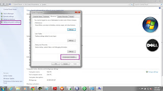
• Go to My Computer -> Properties -> Advanced system Settings

Set the Variables 

JAVA_HOME = C:\Program Files\<Java.exe path>
JRE_HOME=C:\Program Files\Java\<JRE> 
PATH=C:\Informatica\PowerCenter8.6.0\server\bin;

Once the following prerequisites are completed, start the Server installation.
TIP: Browse to the install.exe file and "Run as administrator"
       From the drop-down list, select OS as "Windows Service Pack 3"


Once, the Server setup is completed, go to Services.msc and check the Informatica Services.
If the status is Started, your installation was successful.

Else, close windows firewall and then restart the service.

We will configure and start Repository Services in the next Blog !!
We will also create ODBC connection between Teradata and Informatica.

Please let me know your doubts/comments .

Risk Assessment using Teradata - The use of Mathematical Functions

Mathematical Functions in Teradata:

The following table illustrates the year-on-year transactions of a Loan account. A loan account has the Collateral and the Amount to be paid columns.

If you notice, the area where the Blue indicator(Asset with Bank) goes below the Green Indicator(Amount to  be paid/Risk Exposure), is the Risk-Zone.
If the Customer defaults in this zone, the Bank will have lower assets to recover the loan. This is a classical example of Risk-Management.
All such risks are covered by the BASEL-2 norms.

How Teradata Helps?

Functions in Teradata like SUM and CSUM will help us to effectively calculate the value in the FACTS.
We can decide on these metrics, and then populate the RATE column in the dimension from Real-time Systems.
During FACT populations, the following steps can be performed:

1.  the Current Value of Collateral is calculated
2. The Amount repaid is calculated
3. They are projected over a period.

A Flag can be set in the Report file/Aggregates marking the Customer account as Risky

Example: If the State-run Banks had implemented this strategy, then the defaulting of Kingfisher Airlines could be predicted. A total of INR 50 billion was borrowed by the airline, but the collateral tracking could have saved the day for the Lenders.

Your queries/suggestions are always welcome !!

Difference between Rank() and Row_Number() functions

RANK ():- RANK returns ranking (order) of rows based on the number or expression given in the ORDER BY clause.

ROW_NUMBER ():- It returns the sequential number of the row within a group, starting with 1 based on the ORDER BY clause.

We will see the difference between these 2 functions based on an example:

EMPID	ENAME	SALARY	DEPT_ID	RNK	ROWNUM
1	MATT	1000	10	1	1
4	SHANE	1000	12	1	2
2	SCOTT	2000	10	3	3
7	MARY	2000	10	3	4
3	JEAN	2000	10	3	5
5	DEAN	4000	10	6	6
6	LISA	4000	10	6	7

Now, in a practical scenario, we are required to find the all the employees having Nth highest salary.

In such cases, we can use the below query:

SELECT

  E1

.EMPID

  ,

E1.ENAME

  ,

E1.SALARY

  ,

E1.DEPT_ID

  ,

RANK() OVER(ORDER BY E1.SALARY ASC) AS RNK

  ,

ROW_NUMBER() OVER(ORDER BY E1.SALARY ASC) AS ROWNUM

FROM

TL_62917_DLY1_QRMDB

.EMP1 AS E1

WHERE

(

E1.SALARY =

SELECT

SAL2.SALARY FROM

(

SELECT

SAL1.SALARY,SAL1.RNK FROM

(

SELECT

SALARY,RANK() OVER(ORDER BY SALARY DESC) RNK FROM TL_62917_DLY1_QRMDB.EMP1

GROUP

BY 1

)

SAL1

WHERE

SAL1.RNK= ?RNK

)

SAL2

)

Output for a value of ?RNK =2 will be:

EMPID	ENAME	SALARY	DEPT_ID	RNK	ROWNUM
3	JEAN	2000	10	1	1
2	SCOTT	2000	10	1	2
7	MARY	2000	10	1	3

This query will return Nth salary even if duplicate values are present in the Salary column.

If you look at the above table, 2000 is the 2nd highest salary.